A Programmable Light-Based Computing Architecture and Its Baseline Experiment
Observe. Design. Intervene.
Abstract
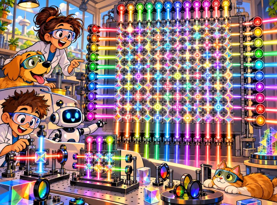
This paper proposes a classical optical computing architecture built as a twelve-by-twelve grid of 144 computational cells. Twelve light emitters feed the grid from the left edge and twelve from the bottom. Twelve receivers sit on the right edge and twelve on the top. Each intersection of a row beam and a column beam is a cell that receives two optical inputs and performs a selectable logic operation on them.
The baseline cell performs one of four Boolean operations: AND, OR, NOR, or XOR. Four is the safe starting point, a set expected to produce a usable result. From there the architecture expands through a wider set of logic functions, then through light levels and stacked spectra, then through degree of polarization, building toward a computing vocabulary far larger than binary.
Readout uses both receiving edges together. The right edge and the top edge each carry half of each cell’s answer, and one additional computation combines the halves to locate and score each cell’s result. Multiple wavelengths make that combination faster and cleaner.
The grid is built on twelves by design. Its 144 cells form a natural base-12 address space, and the architecture favors dozenal organization throughout.
This paper claims no working device. It lays out the architecture, its lineage, its expansion path, and a staged experimental program to test it.
1. The Grid
The system has four arrays on four edges:
- Left edge: twelve programmable emitters, H1 through H12, sending light to the right along twelve rows.
- Bottom edge: twelve programmable emitters, V1 through V12, sending light upward along twelve columns.
- Right edge: twelve receivers, one at the end of each row.
- Top edge: twelve receivers, one at the end of each column.
Twelve rows crossing twelve columns produce 144 intersections. Each intersection is a cell, written C(i,j), where i is the row and j is the column.
A cell doesn’t need its own pair of emitters. It draws its two inputs from the row beam and the column beam that cross at its location. Twenty-four light sources reach 144 cells, much like twenty-four streets laid out in a grid create 144 corners.
Two beams of light passing through each other don’t interact on their own in ordinary materials. Each cell therefore needs an engineered element at the crossing, something that responds to both inputs and produces a readable result. Finding an efficient element is the central engineering problem of the project.
2. Lineage and Prior Art
Parts of this design have relatives going back decades.
Optical crossbar logic arrays. Patents from the late 1980s describe hybrid optical and electronic logic arrays in which a row of emitters sends coded light through a programmable optical crossbar onto a column of detectors, with the result inverted electronically. Those arrays were built to mimic electronic programmable logic arrays, and each crossing acted as an on-off switch rather than a selectable gate.
Optical FPGA elements. In 2009, Nazarathy and colleagues described all-optical gates that can be reprogrammed among AND, OR, XOR, and their inverses by an optical reference signal, and proposed them as building blocks of an all-optical field-programmable gate array. A 2025 study in Micromachines simulated a programmable photonic logic array built from micro-ring resonators.
Photonic crossbars for AI. Researchers now build optical crossbar arrays for the matrix math behind machine learning. Groups have fabricated them at 4×4 and simulated them at 9×9. Those arrays perform weighted multiply-and-add operations, and studies have found that the laser power they need climbs steeply as the grid grows.
Coincident addressing. The readout in Section 7 has an ancestor in magnetic core memory, developed by Jay Forrester at MIT in the early 1950s. Each tiny ferrite ring sat where an X wire crossed a Y wire. Half the switching current went down one wire and half down the other, so only the ring at the crossing received the full amount. Two halves made one answer. Nikolay Brusentsov built his ternary Setun computer from the same kind of ferrite cores.
The 144-cell grid combines pieces of this lineage in a new arrangement: a selectable Boolean gate at each optical row-column crossing, dual-edge readout in which both receiving edges contribute half of each answer, a twelve-based layout, and a planned expansion into multistate light. The searches behind this draft did not turn up that combination in published work.
3. The Baseline: Four Boolean Operations
The first version of the grid supports four operations:
| A | B | AND | OR | NOR | XOR |
|---|---|---|---|---|---|
| 0 | 0 | 0 | 0 | 1 | 0 |
| 0 | 1 | 0 | 1 | 0 | 1 |
| 1 | 0 | 0 | 1 | 0 | 1 |
| 1 | 1 | 1 | 1 | 0 | 0 |
Each cell is assigned one operation, and neighboring cells can run different ones. One cell may run AND while the next runs XOR. With four choices at each of 144 cells, the grid has 4¹⁴⁴, about 5 × 10⁸⁶, possible configurations. That number counts gate arrangements. It does not count independent pieces of input data.
NOR is functionally complete: networks of NOR gates can build any Boolean function. Doing that requires connecting cells to one another, which the baseline grid does not yet do. Routing and feedback come in later stages.
The ceiling above four. With two binary inputs, there are exactly sixteen possible logic functions, and four is a safe subset of them. Published optical gates already reach further. A 2026 Nature Communications device built on an MXene material switches among seven Boolean functions by voltage. A 2024 liquid-metal device reached nine in a single configuration. A 2017 polarization-based gate produced up to twenty-five gate configurations and ran the six basic gates at 1 gigabit per second.
Once the inputs carry more than two states, the count of possible functions grows fast. A cell with two inputs, each holding one of K states, and an output holding one of K states, can perform K^(K²) distinct functions:
| States per signal | Possible two-input functions |
|---|---|
| 2 | 16 |
| 3 | 19,683 |
| 4 | about 4.3 billion |
Combined with stacked light spectra, the upper limit for this architecture is wide open. The baseline stays at four so the first experiment has a clear pass or fail.
4. Why Twelve
Base 10 feels natural because we count on ten fingers. Base 12 designs better. Twelve divides evenly by 2, 3, 4, and 6, so halves, thirds, quarters, and sixths come out as whole numbers. Ten divides cleanly only by 2 and 5. Carpenters, clockmakers, and merchants leaned on twelve for centuries for that reason: inches in a foot, hours on a clock, eggs in a dozen.
The grid builds on twelves at several levels:
- Twelve channels per edge. Inputs can be split into halves, thirds, quarters, or sixths without leftover channels, which makes it easy to divide the grid among several tasks at once.
- A dozenal address space. In base 12, using A for ten and B for eleven, each cell’s address is exactly two digits: row and column. The grid runs from cell 00 to cell BB, with 144 addresses and none wasted. In base 10, the same grid would need awkward addresses from 1,1 to 12,12.
- Twelve output colors. The spectral readout in Section 7 uses twelve output wavelengths, one per row or column.
The baseline experiment runs in binary. The grid’s geometry is dozenal from the start, so later multistate work can move into base 12 without rebuilding the frame.
5. Polarization as the First Signal Alphabet
For the binary baseline, two linear polarizations stand in for the two logic values:
- 0 = horizontal polarization
- 1 = vertical polarization
Both values are lit. A logical zero is horizontally polarized light, and darkness is reserved for a fault: a dead emitter, a broken path, or a missing signal. That separation matters for NOR, which outputs a 1 when both inputs are 0. The cell needs a powered output path so it can produce a lit result even when its inputs both say zero.
The number of polarization states the grid can use beyond two will be measured, not assumed. Each added state has to be produced, carried, and read reliably under real noise.
6. The Computational Cell
Each cell does four jobs:
- Recognize its inputs from the row beam and the column beam.
- Apply its assigned operation.
- Produce a result signal.
- Send the result to both receiving edges.
The first working cell can be a hybrid: detect the two optical inputs, compute the result with a small local circuit, and send the result back out as light. That proves the grid’s addressing, configuration, and readout. It does not prove that light itself performed the logic.
The next step replaces the local circuit with a direct optical element. Candidates include the reconfigurable MXene and liquid-metal gates, polarization-based gates like the 2017 design, and nonlinear materials placed at the crossing. The experimental record has to state plainly where the computation happened in each version, since a hybrid cell and an all-optical cell carry different promises for speed and energy.
7. Readout: Two Halves of One Answer
Each cell reports its result in two directions: along its row toward the right edge, and along its column toward the top edge.
The right-edge receiver for a row holds half the answer, and the top-edge receiver for a column holds the other half. Neither half alone tells you what a given cell did. One additional computation combines the two, and the cell sitting at the crossing of that row and that column is located and scored. It works like magnetic core memory, where half a current on each wire flipped only the core where the wires met.
Keeping inputs and outputs apart. Rows and columns carry inputs in one direction and results in the other. Inputs travel on one wavelength and results on a different one, with filters on the receivers so they read only results.
Stacked spectra make the halves sharper. If the 24 edge receivers only measured total brightness, 24 readings could not separate 144 independent results in a single pass, and the grid would have to read out over several cycles. Color tagging solves that. Each column’s cells send their row-bound result on that column’s own wavelength, and each row’s cells send their column-bound result on that row’s own wavelength. Twelve output colors cover the whole grid, since the row paths and column paths are physically separate and can reuse the same set.
With a spectral splitter in front of it, each right-edge receiver separates the twelve cells in its row by color. Each top-edge receiver does the same for its column. Each cell’s result then shows up twice, once at each edge. The combining step pairs the two readings; agreement confirms the result, and disagreement flags an error in that cell. The grid checks its own work as it reads.
The light budget for this scheme is one input wavelength and twelve output wavelengths.
8. Computational Vocabulary
The long-range aim is a richer physical vocabulary for machine computing. If each cell can hold K distinguishable states, one cell carries log₂(K) bits, and 144 independent cells carry 144 × log₂(K) bits:
| States per cell | Raw capacity across 144 cells |
|---|---|
| 2 | 144 bits |
| 3 | about 228 bits |
| 12 | about 516 bits |
| 16 | 576 bits |
| 256 | 1,152 bits |
These figures assume each cell can be set and read on its own. In the shared-emitter grid, the inputs come from only 24 emitters, so the grid can receive at most K²⁴ distinct input patterns. The 144 cells turn those 24 inputs into 144 relationships between them. They don’t add new information about the inputs themselves.
Those relationships are useful. Machine learning systems spend much of their effort building relationships between input features. Put twelve features on the rows and twelve on the columns, and the grid produces 144 pairwise comparisons in one pass:
- AND flags where two conditions are both present.
- OR flags where at least one is present.
- NOR flags where both are absent.
- XOR flags where two conditions differ.
As cells gain more states and more functions, those comparisons can become graded, layered, and able to carry uncertainty.
9. The Expansion Path
The grid grows in stages, each one tested before the next begins.
Stage One: Four Booleans. AND, OR, NOR, and XOR in binary polarization. This is the baseline expected to produce a usable result.
Stage Two: The Full Boolean Set. Expand each cell toward the full set of sixteen two-input binary functions, building on the seven- and nine-function gates already demonstrated.
Stage Three: Light Levels and Spectra. Vary intensity and add wavelengths so each channel carries more than two states. Stacked spectra multiply the space, the way a radio band carries many stations at once.
Stage Four: Degree of Polarization. Light can be fully polarized, partly polarized, or unpolarized, and the degree can be set like a dial. In August 2026, Petrini, Conti, and Pierangeli reported in Nature that they could program both the polarization state and its degree across more than a thousand spatial channels. This is the expansive version of the grid, where each signal carries a direction and a strength of lean.
Stage Five: The Third Answer. Bright Meadow Group’s companion paper on the Brusentsov Drive proposes ternary logic with a third state, R, meaning “go find the analog answer.” On the grid, R has a natural home in unpolarized light: lit, present, and leaning neither way. Darkness stays reserved for faults.
Part II — Experimental Program
10. Hypothesis
A two-input optical crossing can produce four selectable Boolean operations, and such crossings can be arranged in a 12 × 12 grid using shared inputs and dual-edge readout.
The program climbs in three steps: one cell, then a 3 × 3 array, then the full 12 × 12 grid. Each step has to pass before the next one counts as evidence for the architecture.
11. Experiment A: Single Cell
Apparatus. Two controllable light sources crossing at one point, one horizontal and one vertical, each able to switch between horizontal and vertical polarization. A candidate logic element at the crossing. A way to select among the four operations. Detectors on two edges, with wavelength filters separating inputs from outputs. Data recording, optical shielding, and reference measurements for stray light. Standard optical-bench parts are fine at this stage.
Procedure. For each of the four operations, apply the input pairs 00, 01, 10, and 11, record the output, and compare it against the truth table. Repeat across a range of light powers, switching rates, and room conditions. Measure switching time, separation between output levels, and energy used.
Pass criteria. Four reproducible truth tables, with a provisional target of at least 99 percent correct output for each input pair, followed by tougher reliability testing. Report error rates per input pair, repeatability after reconfiguration, stability as light power changes, electrical energy for control and detection, and optical energy per operation.
12. Experiment B: 3 × 3 Array
Three row emitters and three column emitters create nine cells, each assigned a different operation:
| V1 | V2 | V3 | |
|---|---|---|---|
| H1 | AND | XOR | OR |
| H2 | NOR | AND | XOR |
| H3 | OR | NOR | AND |
Tests:
- Independent configuration: changing one cell’s operation leaves its neighbors alone.
- Shared inputs: cells sharing a row or column each process the shared signal correctly.
- Dual-edge readout: the combining step correctly locates and scores each of the nine cells from the right-edge and top-edge readings.
- Spectral tagging: three output colors separate the three cells on each edge.
- Cross-check: a deliberately faulted cell produces a disagreement between its two readings.
- Crosstalk: stray light and interference between channels are measured.
- Repeatability: the nine-cell configuration holds up through repeated cycles.
13. Experiment C: The Full Grid
Twenty-four emitter channels, twenty-four receiver channels, 144 cells, and twelve output colors.
- Uniform configuration. Set each cell to AND, run several input patterns, and check the 144 outputs. Repeat for OR, NOR, and XOR.
- Mixed configuration. Load a predetermined map of mixed operations and verify each cell.
- Reconfiguration. Change assignments between cycles and measure speed, stability, and errors.
- Parallel readout. Measure how many results the grid delivers per readout interval with spectral tagging, and compare that with the multi-cycle readout needed without it.
- Signal expansion. Once binary performance holds, add one new reliably distinguishable state and test whether it survives the trip through the grid.
14. Energy
Light moves fast, and that alone doesn’t make a system efficient. The energy count has to include the emitters, modulation, cell configuration, any amplification, the receivers and spectral splitters, conversion between analog and digital signals, control electronics, and cooling.
Divide average power during a test run by the number of verified results produced, and compare that figure against a conventional electronic circuit doing the same job. Report speed of light through the grid separately from total time per answer, since the total includes setup, gate operation, readout, and the combining step.
No energy advantage is assumed before it’s measured.
15. Comparison with Conventional Computing
Build a well-optimized digital circuit that takes the same 24 inputs, applies the same gate map, and produces the same 144 results. Run both systems on the same test patterns and compare:
- correct results per second
- time per full grid evaluation
- energy per verified result
- error rate by operation
- reconfiguration time
- hardware complexity
- stability under repeated use
- performance as state counts rise
The test succeeds scientifically even if electronics win. A loss shows which parts need work and which narrower jobs might still suit the optical grid.
16. What Would Force a Rethink
- If the cell can’t tell its input combinations apart, the crossing element needs replacing.
- If the four operations can’t be selected reliably, the cell isn’t yet a programmable gate.
- If the two edge readings can’t be combined to locate cells correctly, the readout scheme needs redesign.
- If spectral tagging adds too much crosstalk between colors, readout may need more cycles and fewer colors.
- If per-cell configuration requires so much extra wiring that the shared-emitter savings vanish, the layout needs rethinking.
- If energy use exceeds a digital equivalent with nothing gained in return, the search shifts to a better-suited application.
- If added states drive error rates too high, the usable alphabet stays small for now.
Results go in the published record either way.
17. Conclusion
The grid starts simple: twelve emitters on two edges, twelve receivers on the other two, 144 crossings, and four logic operations at each crossing. The first experiment asks one narrow question: can two beams of light produce a reliable, selectable logic result where they meet?
If the answer is yes, the grid has a long road ahead. The Boolean set widens toward sixteen functions. Light levels and stacked spectra multiply the states each channel carries. Degree of polarization adds a dial for how strongly a signal leans. The Brusentsov Drive’s third answer finds a home in unpolarized light. The twelve-based frame holds the whole progression together, from the dozenal cell addresses to the twelve output colors.
Speed is the reason people usually reach for light in computing. This grid reaches for it because a single beam can carry color, brightness, polarization, and degree of polarization at once, and each of those can carry meaning. The experiment will show how many of them can be put to work together.
Research status: Proposed architecture and experimental plan. The 144-cell system described here has not been built or independently validated. Published research supports some of its component technologies, not the complete design.
Sources
- All-optical logic processing unit using Kerr nonlinearity of MXene. Nature Communications (2026). https://www.nature.com/articles/s41467-026-70834-0 — summary: https://www.nanowerk.com/spotlight/spotid=69042.php
- All-in-one, all-optical logic gates using liquid metal plasmon nonlinearity. Nature Communications (2024). https://www.ncbi.nlm.nih.gov/pmc/articles/PMC10897469/
- Tang, X., et al. (2017). A Reconfigurable Optical Logic Gate With up to 25 Logic Functions Based on Polarization Modulation With Direct Detection. IEEE Photonics Journal, 9(2). https://doi.org/10.1109/jphot.2017.2684823
- Petrini, A., Conti, C., and Pierangeli, D. (2026). Degree-of-polarization modulation for high-dimensional optical computing. Nature. https://www.ncbi.nlm.nih.gov/pmc/articles/PMC13558076/
- Nazarathy, M., et al. (2009). All-optical linear reconfigurable logic with nonlinear phase erasure. Journal of the Optical Society of America A, 26(8). https://www.doi.org/10.1364/JOSAA.26.000A21
- Programmable Photonic Logic Array Based on Micro-Ring Resonators and All-Optical Modulation. Micromachines (2025). https://doi.org/10.3390/mi16020238
- Tang, R., et al. (2024). Symmetric silicon microring resonator optical crossbar array for accelerated inference and training in deep learning. Photonics Research, 12(8). https://m.researching.cn/articles/OJ577064eada2e7876/figureandtable
- Photonic-Electronic Integrated Circuits for High-Performance Computing and AI Accelerators. arXiv:2403.14806. https://arxiv.org/pdf/2403.14806
- A Case Study on the Performance Metrics of Integrated Photonic Computing. arXiv:2511.00186. https://arxiv.org/pdf/2511.00186
- US Patent 4,926,367. Method and apparatus for programmable optical crossbar logic array with decoders. https://www.patenthub.cn/zhuanli/patent-14289-US4926367A-2e0649a6cceed299f7cfa9f903c82dce.html
- US Patent 4,979,138. High fan factor modified crossbar architecture and method for optical digital computing. https://image-ppubs.uspto.gov/dirsearch-public/print/downloadPdf/4979138